1. Simple moving average

Time series is a stream of data: $x_{1},\, x_{2},\, x_{3},\,\ldots\,,\, x_{k}$ . Here $x_{k}$ is the most recent value. Usually the data are noisy and not smooth. The simplest way to smooth a time series is to calculate a simple moving average [1] of length $n$, which is just the mean of the last $n$ observations: \begin{equation} m_{k}=\frac{1}{n}\sum_{i=k-n+1}^{k}x_{i}\label{eq:mkn} \end{equation} In the beginning, when $k\lt n$, this is a cumulative moving average: \begin{equation} m_{k}=\frac{1}{k}\sum_{i=1}^{k}x_{i}\label{eq:mkk} \end{equation}

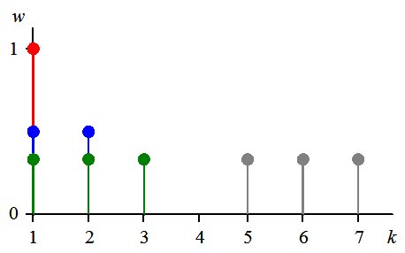
Equal weights, n = 3, k = 1, 2, 3.

Actually Eq. (\ref{eq:mkk}) is the particular case of (\ref{eq:mkn}) for $k=n$. The recurrence for (\ref{eq:mkn}) is \begin{equation} m_{k}=\frac{1}{n}\left[x_{k}+\sum_{i=k-n}^{k-1}x_{i}-x_{k-n}\right]=m_{k-1}+\frac{x_{k}-x_{k-n}}{n}\label{eq:mknr} \end{equation} Similarly for (\ref{eq:mkk}) \begin{equation} m_{k}=\frac{1}{k-1}\left[x_{k}+\sum_{i=1}^{k-1}x_{i}\right]\frac{k-1}{k}=m_{k-1}+\frac{x_{k}-m_{k-1}}{k}\label{eq:mkkr} \end{equation} Note that both (\ref{eq:mknr}) and (\ref{eq:mkkr}) can be rewritten as \begin{equation} m_{k}=m_{k-1}+\frac{\delta_{k}-\delta_{k-n}}{N_{k}}\label{eq:mkur} \end{equation} where \begin{equation} \begin{cases} \delta_{l}=x_{l}-m_{k-1} & l \gt 0\\ \delta_{l}=0 & l\leq0 \end{cases}\label{eq:del} \end{equation} and \begin{equation} \begin{cases} N_{k}=n & ,k\geq n\\ N_{k}=k & ,k\lt n \end{cases}\label{eq:nk} \end{equation} The above unified notations are very convenient for a programming implementation.

2. Exponential smoothing

The simple moving average is the particular case of a weighted average with equal weights. However, it is natural to assign larger weights for recent values and smaller weights for older ones. The exponential smoothing is a popular implementation of this idea. It is defined by the following recurrent relation \begin{equation} \begin{cases} m_{1}=x_{1} & k=1\\ m_{k}=\alpha x_{k}+(1-\alpha)m_{k-1}=\alpha x_{k}+\lambda m_{k-1} & k\gt 1 \end{cases}\label{eq:mker} \end{equation} Here \begin{equation} \lambda=1-\alpha \end{equation} The recurrence (\ref{eq:mker}) also defines a weighted average \begin{equation} m_{k}=\sum_{i=1}^{k}w_{k,i}x_{i}\label{eq:mkw} \end{equation} with the following weights \begin{equation} w_{k,i}=\begin{cases} \lambda^{k} & i=1\\ \alpha\lambda^{k-i} & i \gt 1 \end{cases}\label{eq:wki} \end{equation} The weights decrease exponentially with the decay factor $\nu=-ln(\lambda)$: \begin{equation} \begin{cases} \frac{w_{k,i}}{w_{k,i+1}}=\lambda=e^{-\nu} & i=k-1,\,\ldots,\,2\\ \frac{w_{k,1}}{w_{k,2}}=\frac{\lambda}{\alpha} & i=1 \end{cases}\label{eq:expw} \end{equation} It gave the name for this smoothing.

3. Exponential average

The weight $w_{k,1}$ in (\ref{eq:expw}) does not follow the same exponential rule. For $\lambda>\frac{1}{2}$ it is even not the smallest one. The pure exponential average can be defined as \begin{equation} m_{k}=\frac{S_{k}}{N_{k}} \end{equation} where \begin{eqnarray} S_{k} & = & \sum_{i=1}^{k}\lambda^{k-i}x_{i}\\ N_{k} & = & \sum_{i=1}^{k}\lambda^{k-i} \end{eqnarray}

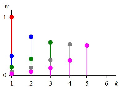
Exponential weights, k = 1, ... , 5.

The above equations can be written as recurrent relations: \begin{eqnarray} S_{k} & = & x_{k}+\lambda S_{k-1}\label{eq:skr}\\ N_{k} & = & 1+\lambda N_{k-1}\label{eq:nkr} \end{eqnarray} Using (\ref{eq:skr}) and (\ref{eq:nkr}), it is easy to derive a recurrence for the mean value \begin{eqnarray*} m_{k} & = & \frac{x_{k}+\lambda S_{k-1}}{N_{k}}\\ & = & \frac{x_{k}}{N_{k}}+\frac{\lambda N_{k-1}}{N_{k}}m_{k-1}\\ & = & m_{k-1}+\frac{x_{k}}{N_{k}}+\left(\frac{\lambda N_{k-1}}{N_{k}}-1\right)m_{k-1}\\ & = & m_{k-1}+\frac{x_{k}}{N_{k}}-\frac{m_{k-1}}{N_{k}} \end{eqnarray*} Finally \begin{equation} m_{k}=m_{k-1}+\frac{\delta_{k}}{N_{k}}\label{eq:mke} \end{equation} where \begin{equation} \delta_{k}=x_{k}-m_{k-1}\label{eq:dele} \end{equation} The equations (\ref{eq:mke}) and (\ref{eq:dele}) are remarkably similar to (\ref{eq:mkur}-\ref{eq:nk}).

4. Effective smoothing length

The smoothing length is well defined in the simple average. It is the norm $N_{k}$ (\ref{eq:nk}). The norm (\ref{eq:nkr}) is the generalization of (\ref{eq:nk}) and defines the effective smoothing length for the exponential average: \begin{equation} N_{k}=\frac{1-\lambda^{k}}{1-\lambda}=\frac{1-\lambda^{k}}{\alpha}\label{eq:norm} \end{equation} This norm accounts for 100 % of all weights. At sufficiently large $k$ \begin{equation} \frac{1}{N_{k}}\rightarrow\frac{1}{N_{\infty}}=\alpha\label{eq:norminf} \end{equation} and $\frac{\lambda^{k-i}}{N_{k}}\approx w_{k,i}$ (\ref{eq:expw}). Therefore both definitions of exponential smoothing coincide for large $k$. Actually the difference between the two definitions tends to zero as $\lambda^{k}$. The definition (\ref{eq:norm}) seems to be natural, however historically the smoothing period $P$ for the exponential smoothing (\ref{eq:mker}) is defined as [2]: \begin{equation} \alpha=\frac{2}{P+1} \end{equation} These two definitions related as \begin{equation} N_{k}=\frac{P+1}{2}\left[1-\left(\frac{P-1}{P+1}\right)^{k}\right]\approx\frac{P+1}{2} \end{equation} In RiskMetrics [ 3] the effective averaging length $L$ is defined as \begin{equation} \frac{N_{L}}{N_{\infty}}=0.999=1-\epsilon \end{equation} Therefore \begin{eqnarray*} 1-\lambda^{L} & = & 1-\epsilon\\ \lambda^{L} & = & \epsilon \end{eqnarray*} or \begin{equation} \lambda=\epsilon^{\frac{1}{L}} \end{equation} This length is related to the natural length as \begin{equation} L=\frac{ln(\epsilon)}{ln(\lambda)} = \frac{ln(\epsilon)}{ln(1-\frac{1}{N_{\infty}})} \end{equation} For $N_{\infty} >> 1$ \begin{equation} L \approx 6.9\; N_{\infty} \end{equation}

In particular, for $\lambda=0.94$ [3], the above definitions give the following values: $L=112$, $P=33$, $N_{\infty}=17$ .  

A couple of specific cases are also worth mentioning. For $N_{\infty}=P=1$ $\lambda=0$ - no averaging; and for $L=1$   $\lambda=0.001$.

The values of all definitions for selected $\lambda$ are collected in the table below.

$\lambda$	L	P	$N_{\infty}$	Comment
0	0	1	1	No averaging
0.001	1	1.002	1.001
0.5	10	3	2
0.75	24	7	4
0.875	52	15	8
0.94	112	33	17	RiskMetrix

Suggested citation for this article:

Nikolai Shokhirev, 2012. Moving Average and Exponential Smoothing, http://www.numericalexpert.com/articles/ma_ewma

References

1. WikipediaMoving average.
2. WikipediaExponential smoothing.
3. Jorge Mina and Jerry Yi Xiao, Return to RiskMetrics: The Evolution of a Standard, RiskMetrics, 2001.