Error: Estimation | Amplification | Propagation

Introduction

The estimation of errors depends on two essential factors: (i) the definition of accuracy and (ii) available information about an error (noise). For example, the statement that the quantity A has the value a ± δa implies that (i) the measure of accuracy is the whole span of values, 2 |δa|, and (ii) the error takes any value from the interval [-δa,  δa]. Note, that this does not specify the distribution of errors within that interval. However, it does imply that the value a does not have a systematic error (is not biased). This itself is a very strong statement, which requires the proof of its validity.

Absolute error rule

Suppose we have two quantities A and B with the values a ± δa and b ± δb, respectively. According to the above definition of accuracy and the  assumption about the errors, ranges of the values of A and B are [ a - |δa|, a + |δa|] and [b - |δb|, b + |δb|]. The range of values of their sum  is

[a + b - |δa| - |δb|, a + b + | δa| + | δb|]

(1)

In other words, the the quantity C = A + B has the value c = a + b and the error |δc| = | δa| + |δb|. From this we can formulate that the absolute errors are always added.

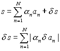
Eq. (1) can be generalized for a weighted sum

(2)

as follows

(3)

Relative errors

A relative error for the quantity C is defined as ηc = | δc| /c. For the case of  a sum of two quantities

ηc = ( | δa| + | δb| )/(a + b)

(4)

The relative error can be very large if a and b are of opposite sign and almost cancel each other.

Variance and Standard deviation

If large errors are relatively rare then some typical errors can be used as a measure of accuracy. A popular choice is the standard deviation. However, the calculation of the standard deviation requires detailed information about the distribution of errors. This means that we have to know the distribution function p(a) (or make some reasonable assumption about p).

The definitions of the standard deviation σ and variance var are

(5)

where

(6)

is the mean value (often denoted as μ or ).

Uniform distribution

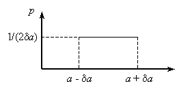
This is the case when all errors within the interval [-δa,  δa] are equally probable:

Fig. 1. The uniform (rectangular) distribution.

The standard deviation is

(7)

For the uniform distribution σ ~ 0.6 δa. The standard deviation does not take into account about 40% of equally probable errors. It means that σ is not quite suitable as a measure of accuracy for this particular error distribution. However   = 1.7320508075688772 σ accounts for 100% of errors.

Normal distribution

The normal distribution, also called Gaussian distribution, is defined as

(8)

Here σ is the standard deviation and μ is the mean value.

This distribution extends to ± infinity and δx cannot be used  as a measure of accuracy. The interval ± σ accounts for 68% of all errors. More values are listed below:

L /σ	P(μ - L < x < μ + L)
1	0.6826894921370859
2	0.9544997361036416
3	0.9973002039367398
4	0.9999366575163338
5	0.9999994266968563
6	0.9999999980268247

Confidence level and interval

From the above table we can tell that 95.4% of all values are in the interval μ ± 2σ. This interval is called the confidence interval and 95.4% is the confidence level. The values μ - 2σ and μ + 2σ are also called the confidence limits.

 

Standard deviation of a sum

Let as present each variable in (2) as its mean value and an error:

A n = a n + ε n.

(9)

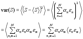
 According to the definition, the variance is

(10)

It can be rewritten as

(11)

Under the assumption that the errors for different variables are independent (uncorrelated) and the covariance can be set to zero in (11). From this we can formulate that the variances of uncorrelated variables are additive.

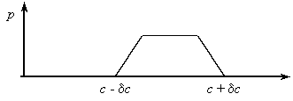
Remark. The distribution of a sum is not necessarily of the same type as for the individual components. For example, the sum of two variables with the uniform distribution (see Fig. 1) has the trapezoidal distribution:

Repeated measurements

The arithmetic mean of N measurements is defined as

(12)

It is also called the population average. Eq. (12) can be considered as a definition of the new random variable with its mean value and variance. The mean value of (12) is the same as for an individual measurement. The variance depends on the way the measurements were made.

If the measurements are independent (uncorrelated) then from (11) we have

(13)

and the standard deviation is

(14)

We can conclude that the repetition of experiments and averaging reduce the error.

 

The N <-> (N - 1) confusion

Sometimes one can see (N - 1) instead of N in denominators of the equations similar to (13-14). There is no contradiction. The above accuracy estimation is based on independent information about the mean values of A (e.g. from a distribution function). In practice, the mean value itself is often estimated as a population average A _mean (12). Then the random variables ΔA _n  = A _n  - A _mean are used for estimation of the variance. The variable ΔA _n  is comprised of two dependent variables because A _mean also contains  A_n . Consider for example the first measurement:

(15)

and

(16)

The correct estimation of the variance is

(17)

For practical variance estimation the following formula is used

(18)

Knowledge is power

The difference between Eqs (13) and (18) reflects the difference in the available information. Eq. (13) is the variance relative to the known mean value. Eq. (18) is the best estimate of the variance along with the estimate of the mean (12). This illustrates the fact that the estimation of errors depends on the information about the random variables.

Error: Estimation | Amplification | Propagation

References

1. Error Analysis.